What a Pangenome Misses, and What It Nails
What a Pangenome Misses, and What It Nails
In my last post I tried to read a Y haplogroup out of a personal pangenome, watched it quietly point me at the wrong branch, and came away with a claim I made mostly by hand-waving: a genotype-only pangenome callset is a panel-conditioned genotyping result, not a complete catalog of your variants, and it misses things silently. I also claimed the graph is strong on structural variation. Both felt true. Neither was measured.
So I measured them. Same WGS229 short-read library and HiFi data, same personal pangenome (T2T-CHM13 plus eight phased assemblies). This time I worked on two whole chromosomes rather than the pathological Y: chr20, a calm and well-behaved autosome, and chr16, one of the most segmental-duplication-rich chromosomes in the genome. I called variants three ways and refereed the hard cases with long reads.
The short version: the trade-off is real, it replicates across an easy and a hard chromosome, and the part I was most confident about is the part I had wrong at first.
The setup
There are three callsets in play, and keeping them straight is the whole game.
- Graph genotype-only. This is
vg callon the pangenome, the thing under test. It genotypes variation that already exists in the graph as nodes and edges, which means variation carried by one of the panel assemblies. - Linear, standard. Map the same reads to linear CHM13, call with GATK HaplotypeCaller. This is the ordinary pipeline a citizen scientist would run, and it discovers variants the reads support whether or not anyone has seen them before.
- Long-read truth. The donor also has PacBio HiFi data. It is only about 4x coverage, which is thin, but long reads are the best independent witness for the hard cases, so I used them as a referee rather than a fourth opinion.
To compare the graph and the linear callset fairly, I surjected the graph alignments back to linear coordinates so the linear caller sees exactly the same reads, then normalized both callsets identically and intersected them. Everything below is on CHM13 coordinates.
The weakness: a silent discovery gap
Start with chr20, the easy case. After normalization the graph emits about 103,000 variants and GATK emits about 106,000. Intersect them and you get three piles:
| Set | chr20 |
|---|---|
| Shared | 79,644 |
| Linear-only (GATK found, graph did not emit) | 26,411 |
| Graph-only (graph emitted, GATK did not) | 23,934 |
A quarter of each callset is unique to it. That is a lot of disagreement on a chromosome that is supposed to be boring. The interesting pile is the 26,411 variants the standard linear pipeline found that the genotype-only graph never emitted. Are those real variants the graph is blind to, or just caller noise?
Two checks answer it.
First, can the graph even represent them? I ran vg deconstruct to enumerate every variant carried by any panel assembly on chr20, then asked how many of the linear-only variants are present anywhere in that panel. The answer is brutal: 26,116 of 26,411, or 98.9 percent, are absent from the panel entirely. The graph could not have called them no matter how good the genotyper was, because the alleles are simply not in it. Only 295 were representable-but-missed, so when the graph can represent something it genotypes it almost perfectly. The gap is not a sensitivity problem. It is a representation problem.
Second, are they real, or is GATK inventing them? Here is where the HiFi referee earns its keep. I pulled the HiFi pileup at every SNP and asked what fraction show the alternate allele in at least one long read, using the variants both callers agree on as a real-variant baseline.
| SNP set | HiFi-covered | alt allele confirmed |
|---|---|---|
| Shared (real baseline) | 93.8% | 88.3% |
| Linear-only (the discovery gap) | 82.4% | 65.0% |
| Graph-only | 48.0% | 43.0% |
The linear-only variants confirm at 65 percent against an 88 percent ceiling for known-real variants. They are mostly real. The 26,000-variant discovery gap is genuinely missed private variation, not GATK fantasy.
And notice the bottom row, because it is the other half of the story. The graph-only calls, the ones the graph emits that GATK does not, confirm at only 43 percent, and barely half of them even have HiFi coverage. They sit in regions where reads do not map cleanly, and most of them do not reproduce. The graph is not just missing real variants. It is also inventing artifacts in the hard regions, the same paralog-collapse problem that wrecked the Y. So the genotype-only graph fails in both directions at once: it cannot see your private variation, and it over-calls noise where the reads are ambiguous.
This is why I keep harping on the word “silently.” In a sites-only graph VCF, an absent record could mean the sample matches the reference, or the allele is not in the graph, or there was no coverage. Three completely different situations, one indistinguishable blank. A linear caller at least tells them apart.
The strength: structural variants, and a lesson in being wrong
Now the other claim. Pangenomes are supposed to shine at structural variation, the insertions and deletions and rearrangements a single linear reference handles worst. The graph does carry a lot of large alleles inline. On chr20 it emits 976 variants of at least 50 base pairs, all the way up to a 144 kilobase allele, sitting right there in the same callset as the SNPs.
My first instinct was to compare that against GATK and declare victory. GATK found 122 variants of 50 base pairs or more. Graph 976, linear 122, done.
That was wrong, and it is worth saying why, because it is a trap. GATK HaplotypeCaller is a small-variant caller. Structural variants in the GATK world are an entirely separate pipeline. HaplotypeCaller does local assembly in small windows and has a hard ceiling on event size. When I plotted the size distribution, every single one of its 122 “large” calls was under 300 base pairs. It produces nothing bigger, by design. Comparing the graph’s SVs to HaplotypeCaller’s is comparing a structural variant caller to a tool that cannot call structural variants. I retracted the number.
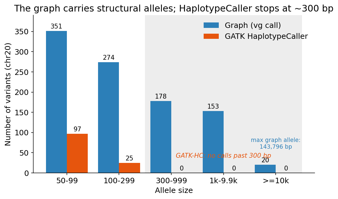 Large-allele size distribution on chr20. The graph carries structural alleles across every size band out to 144 kb, while GATK HaplotypeCaller produces nothing past 300 bp. It is not a less sensitive SV caller, it is not an SV caller.
The fair comparison needs a real short-read SV caller, so I built Delly from source (no package for it on this machine) and ran it on a proper bwa-mem alignment of the same reads. Delly is the actual linear SV workflow: paired-end and split-read signals, the works. On chr20 it calls 313 structural variants.
So now it is 976 graph alleles versus 313 Delly calls, which sounds like the graph still wins, except the two barely agree. Only about a third of Delly’s calls land near a graph allele, and only about a fifth of the graph’s larger SVs land near a Delly call, and widening the breakpoint window to a full kilobase barely moves either number. They are finding different things. At this point my honest conclusion was deflating: structural variant calling is a mess, the two methods disagree badly, and neither is obviously right.
The HiFi referee breaks the tie, and it breaks it hard in the graph’s favor.
| chr20, against HiFi-validated SVs | recovered |
|---|---|
| Graph | 274 / 338 (81%) |
| Delly (short read) | 88 / 338 (26%) |
When long reads confirm a structural variant, the graph has it 81 percent of the time and short-read Delly has it 26 percent of the time. The low graph-versus-Delly agreement was not two equal views disagreeing. It was Delly missing most of the real SVs. Short reads are especially blind to insertions, which makes sense, since a short read cannot span an insertion longer than itself. HiFi found 156 insertions on chr20. Delly found 22.
So the graph really is better at structural variation, but I only got to say so after taking the long way around: a retracted number, a compiler, and a long-read reality check. I will take an honest yes over a lucky one.
There is one caveat I want to leave standing. At 4x, HiFi confirms presence well but cannot establish absence. Most graph SV calls are not HiFi-confirmed, but at 4x most real SVs would not be either, so I cannot estimate the graph’s structural false-positive rate from this data. The graph’s SV sensitivity is established. Its SV precision is not, and judging it would need deeper long reads.
The hard chromosome
One chromosome is an anecdote. The whole point of picking chr16 was that segmental duplications are exactly where you expect a graph to help and short reads to fail, so it is the chromosome most likely to either confirm the story or break it.
It confirmed it, and it sharpened the best part.
| chr20 (easy) | chr16 (segdup-rich) | |
|---|---|---|
| Representation gap (discovery gap not in panel) | 98.9% | 98.8% |
| Discovery-gap SNPs HiFi-confirmed (real) | 65% | 60% |
| Graph-only SNPs HiFi-confirmed (artifacts) | 43% | 43% |
| HiFi-SV recovery, graph | 81% | 77% |
| HiFi-SV recovery, Delly (short read) | 26% | 14% |
The discovery gap is rock steady: about 99 percent representation gap, about two thirds real, on both the easy and the hard chromosome. The graph’s artifact rate is a stable 43 percent on both. Neither of those was a chr20 fluke.
The structural variant gap, though, widens. Short-read Delly falls from 26 percent down to 14 percent recovery in the segmental duplications, because that is precisely where paired-end and split-read signals fall apart. The graph barely flinches, holding at 77 percent. The graph-to-Delly sensitivity ratio grows from about three to one on the easy chromosome to about five to one on the hard one. The harder the region, the bigger the pangenome’s structural-variation edge. That is the most satisfying number in the whole experiment, because it is the one biology predicts.
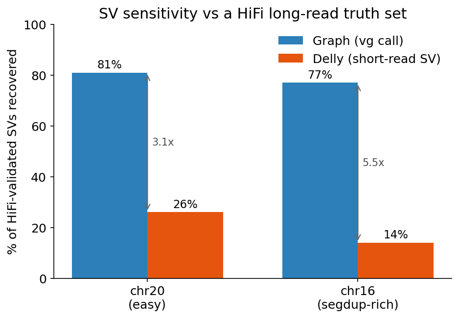 Fraction of HiFi-validated structural variants each method recovers, on the easy chromosome (chr20) and the segmental-duplication-rich one (chr16). The graph holds near 80 percent in both. Short-read Delly is weak on chr20 and collapses on chr16, so the gap widens exactly where the regions get hard.
What it adds up to
Two chromosomes, deliberately the easiest and one of the hardest, tell the same story:
- The pangenome’s weakness is SNP discovery. A genotype-only graph callset cannot see variation that is not in its panel, which is most of your private variation, and it says nothing about the omission. It also over-calls artifacts in repetitive regions. For finding small variants, an ordinary linear caller is simply the better tool.
- The pangenome’s strength is structural variation, and it is a real strength, validated by long reads, and it grows in exactly the difficult regions where you need it most. Short-read SV calling is the weak link there, not the graph.
For anything built on top of this, the operating rule writes itself. Do not treat a genotype-only graph VCF as a finished callset. For small-variant discovery, surject the reads to linear and call them normally, or augment the graph with the reads first. But for structural variation, the graph is the place to look, and the more repetitive the neighborhood, the more that is true.
The first post ended by saying a genotype-only pangenome callset is a panel-conditioned genotyping result wearing the costume of a variant catalog. I believe that more now, with receipts. What I did not expect was how cleanly the same experiment would also show where the graph is not just adequate but genuinely the right tool. The trade-off is not “pangenomes good” or “pangenomes bad.” It is “pangenomes for structure, linear for discovery,” and now I can point at the numbers.